
Data note. This case study uses a synthetic e-commerce dataset of 250,000 customers, built to be realistic in structure. In it, website and app engagement is a leading signal of churn by construction, so the model finding it shows that the pipeline works, not anything about a real business.
The question
How much will each active customer spend over the next 12 months, how sure are we, why, and who should the business look at first? A single average lifetime value can't answer that, because it describes a typical customer who doesn't exist. This project forecasts each customer separately and reports the uncertainty around every forecast.
Data and setup
The synthetic world has 250,000 customers, 2.36 million orders, 4.0 million order lines, 7.2 million engagement rows and 102,000 service tickets across 48 months, with 28 automated data-quality checks. From it I built 62 point-in-time features in SQL (recency, frequency and spend, order cadence and momentum, discount dependency, returns, engagement and service contacts).
Validation: testing on a year the models never saw
Customer value is a forecast about the future, so the check has to be on the future. I used three snapshot dates (30 June 2023, 2024 and 2025) for training, validation and test. Each label is the following 12 months of revenue, and the label windows never overlap. Models were tuned on the validation year only, and the test year was used once.
Leakage is where CLV projects most often go wrong, so the leakage controls are tested, not just described:
- Only rows dated on or before the snapshot are read.
- A return counts only if it was processed by the snapshot date.
- A test confirms that features at the snapshot are identical when every later row is deleted.
- Customer IDs are shuffled so the ID carries no information about acquisition order.
Results on the unseen test year
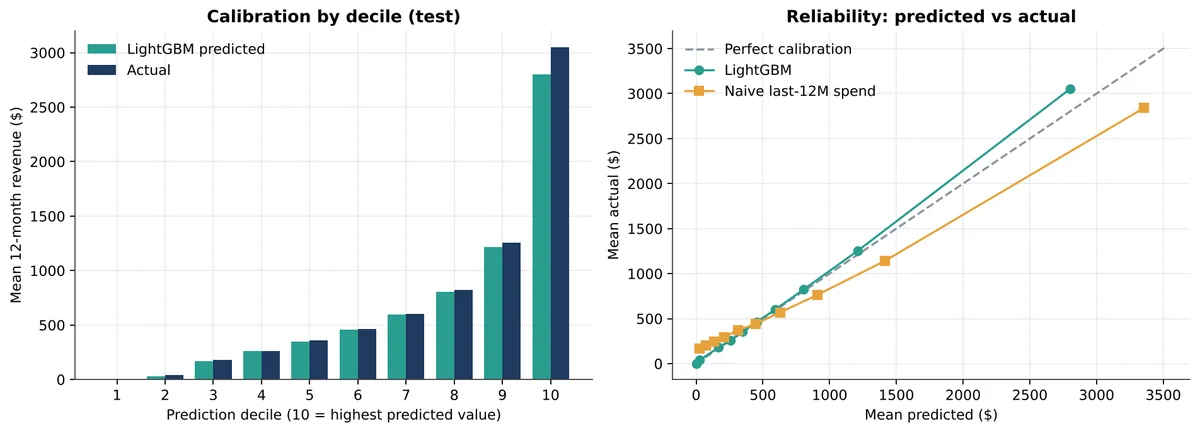
The test set was 126,337 customers, with features as of 30 June 2025 and revenue measured over the following 12 months.
| Model | MAE | R² | Top-10% capture* |
|---|---|---|---|
| LightGBM (Tweedie) | $439 | 0.587 | 43.4% |
| LightGBM (squared error) | $451 | 0.581 | 43.3% |
| Random forest | $454 | 0.566 | 43.1% |
| Baseline: next year = last year | $543 | 0.520 | 40.4% |
| Elastic net | $503 | 0.464 | 42.3% |
| Baseline: training mean | $745 | −0.003 | 9.7% |
*Share of all next-year revenue earned by the 10% of customers the model ranks highest. A perfect ranking would capture 52.6%.
- LightGBM beat the "same as last year" baseline by $104 of error per customer (paired bootstrap 95% interval: $101 to $107).
- The gain repeated on three further synthetic worlds with different random seeds: 18–20% lower error than the baseline.
- A separate purchase-propensity model (will the customer buy in the next 90 days) reached ROC-AUC 0.840 and was well calibrated (ECE 0.008).
An honest ceiling
Because the data is simulated, I could also build an oracle that knows each customer's true hidden purchase rate and whether they are still active. It reaches R² 0.85. That leaves real room above 0.59, but it also shows that a large share of next-year spend can't be predicted from behaviour alone. I describe 0.59 as useful, not excellent.
Giving every forecast a range
Split-conformal prediction intervals were calibrated on held-out data. The 80% intervals covered 80.4% of test customers, with a median width of about $996. Coverage isn't even across groups: it ran from about 98% in the lowest predicted decile to about 75% in the highest, so for the very top customers the interval is a rough guide rather than a guarantee.
From forecast to decision
Each customer was placed in one of six segments using predictions only, and the segments were then compared with what actually happened in the test year.
| Segment | Customers | Last-12-month spend | Predicted change | Actual change |
|---|---|---|---|---|
| Rising star | 24,214 | $11.5M | +82% | +83% |
| Core high-value | 9,504 | $21.3M | −4% | +3% |
| High-value, deteriorating | 9,599 | $28.3M | −29% | −22% |
| Growth opportunity | 14,663 | $12.7M | −22% | −18% |
| Low-value steady | 34,045 | $9.4M | −14% | −10% |
| Fading / lapsing | 34,312 | $11.7M | −58% | −57% |
The ordering is right, and the "deteriorating high-value" group really did lose about a fifth of its revenue. The model is somewhat too pessimistic about declines (−29% predicted against −22% actual). SHAP values explain each forecast in plain language, for example which behaviours pushed a customer's forecast up or down.
Limitations
- The data is synthetic. Real behaviour is messier.
- Total test-year revenue was under-predicted by 5.2%, and more for long-tenured customers. A model trained on past years doesn't fully anticipate growth.
- The model forecasts customers who bought in the last 12 months. In the test year those customers produced 77% of next-year revenue; 22% came from customers acquired after the snapshot, so new-customer revenue needs its own forecast.
- The recommended actions are rules, not causal estimates. There is no A/B data here, so I make no return-on-investment claim.
How I would apply this to your data
For a real shop or subscription business I need an order history with customer IDs and dates, plus refunds if you have them. Engagement and support data improve the forecast but aren't required. The result is a scored customer table with a forecast, a range and the main reasons for each customer, and a short note on how far to trust it. For background on the method, see how to model customer lifetime value and trust the result. The code, 38 automated tests, model card and a live demo are public: predictive-customer-lifetime-value on GitHub and the interactive dashboard (demonstration data).